In-Network Learning for Distributed RAN AI

1 Distributed Inference over Wireless RANs

Wireless radio access networks (RANs) have important intrinsic features that may pave the way for crossfertilization between machine learning (ML) and communication. This is in contrast to simply replacing one or more communication modules by applying ML algorithms as black boxes. For example, while relevant data is generally available at one point in areas such as computer vision and neuroscience, it is typically highly distributed across several sites in wireless networks. Examples include channel state information (CSI) or the socalled radio-signal strength indicator (RSSI) of a user's signal, which can be used for things like localization, precoding, or beam alignment.

A common approach for implementing ML solutions in wireless networks involves collecting all relevant data at one site (e.g., a cloud server or macrobase station) and then training a suitable ML model using all available data and processing power. However, this approach may not be suitable in many cases due to the large volumes of data and the scarcity of network resources, such as power and bandwidth. Additionally, some applications (e.g., automatic vehicle driving) might have stringent latency requirements that are incompatible with data sharing. In other cases, it might be desirable to not share the raw data in order to protect user privacy. Furthermore, edge devices such as small base stations, on-board sensors, and smartphones typically have limited memory and computational power. Also, the wireless environment is typically prone to rapid changes, for example, connectivity fluctuations or devices dynamically joining or leaving the network. Another critical aspect is that the data is largely multimodal, heterogeneous, or both across devices and users. Table 1 summarizes the main features of inference over wireless RANs.

1.1 AI at the Wireless Edge

The challenges discussed earlier have called for a new paradigm, referred to as "edge learning" or distributed learning, in which intelligence moves from the heart of the network to its edge. In this new paradigm, communication plays a central role in the design of efficient ML algorithms and architectures because both data and computational resources, which are the main ingredients of an efficient ML solution, are highly distributed. The goal of distributed inference over RAN is to make decisions on one or more tasks, at one or more sites, by exploiting the available distributed data. In this framework, multiple devices (e.g., BSs and UEs) are each equipped with a neural network (NN). Some of the devices possess data they have acquired through communication or sensing, whereas some only contribute to the collective intelligence through computational power. See Figure 1.

Figure 1 Distributed inference over wireless RAN

1.2 A Brief Review of SOTA Algorithms

AI solutions for RANs can be classified according to whether only the training phase is distributed (such as Horizontal Federated Learning and Horizontal Split Learning) or both the training and inference (or test) phases are distributed (such as Vertical Federated Learning).

Table 1 Summary of the main features of inference over wireless RAN

• Horizontal Federated Learning (HFL): Perhaps the most popular distributed learning architecture is HFL. This architecture, as already mentioned, is most suitable for settings in which the training phase is performed in a distributed manner while the inference phase is performed centrally. During the training phase, each client is equipped with a distinct copy of a same NN model that the client trains on its local dataset. The learned weight parameters are then sent to and aggregated by (e.g., their average is computed) a cloud server or parameter server (PS). This process is repeated, each time using the obtained aggregated model for reinitialization, until convergence. The rationale is that this approach ensures the model is progressively adjusted to account for all variations in the data, not only those of the local dataset.
• Vertical Federated Learning (VFL): In VFL, a variation of Federated Learning (FL), the data is partitioned vertically and both the training and inference phases are distributed. Figure 2 illustrates both HFL and VFL. In this case, every client holds data that is relevant for a possibly distinct feature. A prominent example is when the data is heterogeneous across clients or multimodal. In VFL, different clients may apply distinct NN models that are better tailored for their own data modalities. These models are trained jointly to extract features that collectively are enough to make a reliable decision at the fusion center. An illustration is given in Figure 3a.

Figure 2 HFL (left) and VFL (right)

• Split Learning (SL): SL was introduced in. Similar to FL, it has two variations: Horizontal SL (HSL) and Vertical SL (VSL). Although VSL was introduced earlier than VFL, VSL is now viewed as a special case of VFL. As such, we will not discuss it here. For HSL, a two-part NN model is split into an encoder part and a decoder part. Each edge device possesses a copy of the encoder part and both NN parts are learned sequentially. The decoder does not have its own data, whereas in every training round, the NN encoder part is fed with the data of one device and its parameters are initialized using those learned from the previous round. Then, during the inference phase, the learned two-part model is applied to centralized data.

Figure 3 Feature redundancy removal by INL

2 In-Network Learning

2.1 Overview

INL is most suited to distributed inference from heterogeneous and multimodal data. In this scheme, every device is equipped with an NN. During inference, each device independently extracts suitable features from its input data for a given inference task. These features are then transmitted over the network and fused at a given fusion center in order for a desired reliable decision to be made. The devices that hold useful data (these devices play the role of encoders ) perform individual feature extraction independently from each other. Through training, the algorithm ensures that the encoders only extract complementary features and that, for instance, redundant inter-device features are removed, enabling substantial bandwidth savings. In summary, the key technical components of this algorithm are as follows:

• Network Feature Fusion: INL fuses features that are extracted in a distributed manner at a fusion center so that, collectively, they enable a desired decision to be made at the fusion center after being transmitted over the network.
• Feature Redundancy Removal: A distinguishing factor of INL is that, during inference, the encoders only extract non-redundant features and are trained to do so during training. Specifically, during inference, each encoder only extracts features that are useful for a given inference task from its input data while also taking into account the other features extracted by other encoders.
• Feature Extraction Depends on Network Channel Quality: Encoder feature extraction also takes into account the quality of the channel to the fusion center. That is, features are extracted only to the extent that it is possible to transmit them reliably to the decision maker.
• Satellite Decoders: The fusion center is equipped with a main decoder and satellite decoders, which are trained to make soft decisions based on the individual features transmitted by the encoders. The system is depicted in Figure 3b.

2.2 Formal Description

We model an N-node network by a directed acyclic graph G = (N, E, C), where N = [1 : N] is the set of nodes, \( E \in N ×N\) is the set of edges, and \(C = {C_{jk} : (j, k) ∈ E }\) is the set of edge weights. Each node represents a device, and each edge represents a communication channel with capacity \(C_{jk}\). The processing at the nodes of the set J is such that each of them assigns an index or message \( m_{jl} ∈ [1,M_{jl}]\) to each \(（x_{j} ∈ X-{j}）\) and each received index tuple \((m_{i j} : (i, j) ∈ E)\) for each edge \( ( j, l) ∈ E \). Specifically, let for j ∈ J and l such that \(( j, l ) ∈ E\) the set \(（M_{jl} = [1 : M_{jl}] \). The encoding function at node j is

\( \phi_{j} : X_{j}\times \left \{ {\LARGE \times } _{i:(i, j) \in \mathcal{E}} \mathcal{M}_{i j} \right \} \longrightarrow {\LARGE \times }_{l:(j, l) \in \mathcal{E}} \mathcal{M}_{j l}\)         (1)

where \({\LARGE \times }\) designates the Cartesian product of sets. Similarly, for \(k \in[1:N-1]/J\) , node k assigns an index \(m_{kl} ∈ [1,M_{kl}]\) to each index tuple \((m_{ik} : (i, k) ∈ E)\) for each edge \((k, l) \in E\). That is,

\( \phi_{k} : {\LARGE \times }_{i:(i, k) \in \mathcal{E}} \mathcal{M}_{i k} \longrightarrow {\LARGE \times }_{l:(k, l) \in \mathcal{E}} \mathcal{M}_{k l}\)         (2)

The range of the encoding functions \(ϕ_{i}\) are restricted in size, as

\( \log \left|\mathcal{M}_{i j}\right| \leq C_{i j} \quad \forall i \in[1, N-1] \quad \text { and } \quad \forall j:(i, j) \in \mathcal{E} \)         (3)

Node N needs to infer on the random variable \(Y ∈y\) using all incoming messages, specifically

\( \psi: {\LARGE \times }_{i:(i, N) \in \mathcal{E}} \mathcal{M}_{i N} \longrightarrow \hat{y} \)          (4)

We choose the reconstruction set \(\hat{Y}\) to be the set of distributions on Y, where \(\hat{Y}= P(Y)\). We also measure discrepancies between true values of Y ∈ Y and their estimated fits in terms of average logarithmic loss, specifically for \((y, \hat{P} )\in y\times p(Y)\)

\(d(y ,\hat{P})=log\frac{1}{\hat{P}(y)}\)          (5)

As such, the performance for a given network topology and bandwidth budget \(C_{ij}\) in INL is measured by the achieved relevance level, evaluated as

\(\Delta =H(Y)-E\left [ d(Y,\hat{Y}) \right ] \)          (6)

For example, for classification problems, the relevance measure (6) is directly related to the miss-classification error.

In practice, in a supervised setting, the mappings given by (1), (2), and (4) need to be learned from a set of training data samples \(\{(x_{1,i},...,x_{J,i},y_i)\}_{i=1}^n\). The data is distributed such that samples \(x_{j} := (x_{j},1,..., x_{j},n)\) are available at node j for \(j \in J\) and the desired predictions \( y := (y_{1},..., y_{n})\) are available at the end decision node N. We parametrize the possibly stochastic mappings (1), (2), and (4) using NNs, which can be arbitrary and independent. For example, unlike in FL, these NNs do not need to be identical. It is only required that the following mild condition be met (this condition, as will become clearer from what follows, facilitates the back-propagation). For \(j \in J \) and \(x_{j}\in \mathcal {X_j}\) (We assume all the elements of \(X_{j}\) have the same dimension )

Size of first layer of \( NN (j) = Dimension(x_{j})+\sum_{i:i,j{\scriptsize \in} { \varepsilon } }\)(Size of last layer of NN (i))      (7)

Similarly, for \(k∈[1 : N ]/J\), we set Size of first layer of \(NN (k) =\sum_{i:i,k{\scriptsize \in} { \varepsilon } }\) (Size of last layer of NN (i)).      (8)

In the following, without loss of generality, we illustrate the training and inference phases formally for the example network topology shown in Figure 4.

Figure 4 INL for an example RAN

1. Training Phase: During the forward pass, every node \( j \in {1, 2, 3}\) processes mini-batches of its training dataset \(x_{j}\). The size of these mini-batches is \(b_{j}\). Nodes 2 and 3 send their vectors formed of the activation values of the last layer of their NNs to node 4, where the vectors are concatenated vertically at the input layer of NN 4, due to (7). The forward pass continues on the NN at node 4 until its last layer. Next, nodes 1 and 4 send the activation values of their last layers to node 5. Again, as the sizes of the last layers of the NNs of nodes 1 and 4 satisfy (8), the sent activation vectors are concatenated vertically at the input layer of NN 5. Likewise, the forward pass continues until the last layer of NN 5. All nodes update their parameters using a standard back-propagation technique, as follows. For node t ∈ N, let \(L_{t}\) denote the index of the last layer of the NN at node t. Also, let, for \(\mathbf{w} _{t}^{[l]} \), \(\mathbf{b} _{t}^{[l]} \) and \(\mathbf{a} _{t}^{[l]} \) denote respectively the weights, biases, and activation values at layer \(l ∈ [2 : L_{t}]\) for the NN at node t. \(\sigma\) is the activation function, and \(\mathbf{a} _{t}^{[l]} \) denotes the input to the NN. Node t computes the error vectors

\(\boldsymbol{\delta}_{t}^{\left[L_{t}\right]}=\nabla_{\mathbf{a}_{t}^{\left[L_{t}\right]}} \mathcal{L}_{s}^{N N}(b) \odot \sigma^{\prime}\left(\mathbf{w}_{t}^{\left[L_{t}\right]} \mathbf{a}_{t}^{\left[L_{t}-1\right]}+\mathbf{b}_{t}^{\left[L_{t}\right]}\right)\)         (9a)

\(\boldsymbol{\delta}_{t}^{[l]}=\left[\left(\mathbf{w}_{t}^{[l+1]}\right)^{T} \boldsymbol{\delta}_{t}^{[l+1]}\right] \odot \sigma^{\prime}\left(\mathbf{w}_{t}^{[l]} \mathbf{a}_{t}^{[l-1]}+\mathbf{b}_{t}^{[l]}\right) \forall l \in\left[2, L_{t}-1\right]\)         (9b)

\(\boldsymbol{\delta}_{t}^{[1]}=\left[\left(\mathbf{w}_{t}^{[2]}\right)^{T} \boldsymbol{\delta}_{t}^{[2]}\right] \)         (9c)

and then updates its weight- and bias-parameters as

\(\begin{aligned} \mathbf{w}_{t}^{[l]} & \rightarrow \mathbf{w}_{t}^{[l]}-\eta \delta_{t}^{[l]}\left(\mathbf{a}_{t}^{[l-1]}\right)^{T}, \end{aligned}\)         (10a)

\(\begin{aligned} \mathbf{b}_{t}^{[l]} & \rightarrow \mathbf{b}_{t}^{[l]}-\eta \boldsymbol{\delta}_{t}^{[l]} \end{aligned} \)         (10b))

where \(\eta \) designates the learning parameter(For simplicity, \(\eta \) and \(\sigma\) are assumed here to be identical for all NNs).

During the backward pass, each NN updates its parameters according to (9) and (10). Node 5 is the first to apply the back-propagation procedure in order to update the parameters of its NN. It applies (9) and (10) sequentially, starting from its last layer.

Figure 5 Forward and backward passes for the network topology of Figure 4

The error propagates back until it reaches the first layer of the NN of node 5. Node 5 then horizontally splits the error vector of its input layer (9c) into 2 sub-vectors. The size of the top sub-error vector is that of the last layer of the NN of node 1, and the size of the bottom sub-error vector is that of the last layer of the NN of node 4 — see Figure 5. Similarly, the two nodes 1 and 4 continue the backward propagation during their turns simultaneously. Node 4 then horizontally splits the error vector of its input layer (9c) into 2 sub-vectors. Likewise, the size of the top sub-error vector is that of the last layer of the NN of node 2, and the size of the bottom sub-error vector is that of the last layer of the NN of node 3. Finally, the backward propagation continues on the NNs of nodes 2 and 3. The entire process is repeated until convergence.

2. Inference Phase: During inference, nodes 1, 2, and 3 observe (or measure) each new sample. Let \(x_{1}\), \(x_{2}\) and \(x_{3}\) be the samples observed by nodes 1, 2, and 3, respectively. Node 1 processes \(x_{1}\) using its NN and sends an encoded value \(u_{1}\) to node 5; similarly, nodes 2 and 3 send their encoded values towards node 4. Upon receiving \(u_{2}\) and \(u_{3}\) from nodes 2 and 3, node 4 concatenates them vertically and processes the obtained vector using its NN. The output \(u_{4}\) is then sent to node 5. The latter performs similar operations on the activation values \(u_{1}\) and \(u_{4}\). This node then outputs an estimate of the label y in the form of a soft output \(Q_{\phi _{5}}(y|u_{1},u_{4})\).

3 Performance Gains

In this section, we compare the algorithms HFL and VFL, SL, and our INL for data classification problems, in terms of achieved accuracy and bandwidth requirements.

3.1 INL vs. HFL and HSL

Experiment 1: We create five sets of noisy versions of images obtained from the CIFAR-10 dataset. The images are first normalized, and they are then corrupted by additive Gaussian noise with standard deviation set respectively to 0.4, 1, 2, 3, 4. For INL, each of the five input NNs is trained on a different noisy version of the same image. Each NN uses a variation of the VGG network, with the categorical cross-entropy as the loss function. The architecture is shown in Figure 6. In the experiments, all five noisy versions of every CIFAR-10 image are processed simultaneously, each by a different NN at a distinct node.

Figure 6 Network architecture. Conv stands for a convolutional layer, and FC stands for a fully connected layer.

Subsequently, the outputs are concatenated and then passed through a series of fully connected (FC) layers at node (J + 1). For HFL, each of the five client nodes is equipped with the entire network of Figure 6. The dataset is split into five sets of equal sizes, with the split being performed such that all five noisy versions of a given CIFAR-10 image are presented to the same client NN (note, however, that distinct clients observe different images).

For HSL, each input node is equipped with an NN formed by all five branches with convolution networks (i.e., the entire network shown in Figure 6, except the part at Node (J + 1)). Furthermore, node (J + 1) is equipped with fully connected layers at Node (J + 1) in Figure 6. Here, the processing during training is such that each input NN vertically concatenates the outputs of all convolution layers and then passes that to node (J + 1), which then propagates back the error vector. After one epoch at one NN, the learned weights are passed to the next client, which performs the same operations on its part of the dataset.

Figure 7 shows the amount of data needed to be exchanged among the nodes (i.e., bandwidth resources) in order to get a prescribed value of classification accuracy. Observe that our INL requires significantly less data transmission than HFL and HSL for the same desired accuracy level.

Figure 7 Accuracy vs. bandwidth cost for Experiment 1

Experiment 2: In the previous experiment, the entire training dataset was partitioned differently for INL and HFL in order to account for their unique characteristics. In this second experiment, they are all trained on the same data. Specifically, each client NN sees all CIFAR-10 images during training, and its local dataset differs from those seen by other NNs only by the amount of added Gaussian noise (standard deviation chosen respectively as 0.4, 1, 2, 3, 4). Also, to ensure a fair comparison of the three schemes, INL, HFL, and HSL, we set the nodes to utilize the same NNs fairly for each of them. See Figure 8.

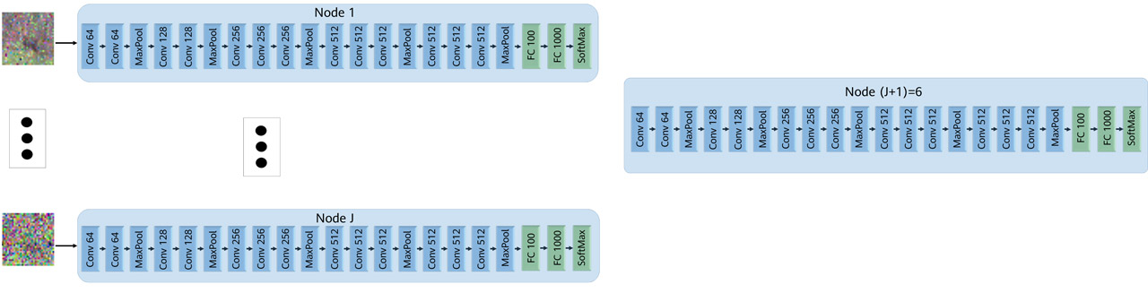
Figure 8 Used NN architecture for Experiment 2

Figure 9 shows the performance of the three schemes during the inference phase in this experiment. For HFL, the inference is performed on the image whose quality is the average among the five noisy input images used for INL. Again, observe the benefits of INL over HFL and HSL in terms of both achieved accuracy and bandwidth requirements.

Figure 9 Accuracy vs. bandwidth cost for Experiment 2

3.2 INL vs. VFL

Experiment 3: In our third experiment, we compare our INL with VFL (as mentioned earlier, VSL can be viewed as a special case of VFL). We use variations of the CIFAR-10 dataset. In particular, we consider two encoders and one decoder, which communicate over a wireless network with a channel capacity of \( R_{1}\) bits per channel used from Encoder 1 to the decoder and \( R_{2}\) bits per channel used from Encoder 2 to the decoder (see Figure 3b). The dimension of the latent vectors \( U_{1}\) and \( U_{2}\) is set to 64. At every time point during the inference phase, the input of the first encoder is a half-occluded copy of a given CIFAR-10 image, and that of the second encoder is a noisy version of the same image. The encoders use CNNs with a few convolutional layers or ResNet-18. The decoders consist of FC layers.

As shown in Figure 10 for CNN encoders and in Figure 11 for ResNet-18 encoders, VFL requires around three times more bandwidth than our INL in order to reach the same AI service accuracy. For some values of accuracy, the advantage of INL in terms of communication cost saving can be significantly higher. Moreover, for a bandwidth of R\( R_{1} = R_{2} = 20\) bits/sample, INL already achieves 45% accuracy, whereas VFL achieves only 28%.

Figure 10 Performance gains of INL vs. VFL for Experiment 3 using CNN encoders

Figure 11 Performance gains of INL over VFL for Experiment 3 using ResNet-18 encoders

4 LLM

In addition to having remarkable capabilities, large language models (LLMs) are revolutionizing AI development and potentially shaping our future. However, their multimodality, in part, causes some critical challenges for cloud-based deployment: (i) long response time, (ii) high communication bandwidth cost, and (iii) infringement of data privacy. As a result, there is an urgent need to leverage Mobile Edge Computing (MEC) in order to finetune and deploy LLMs on or in closer proximity to data sources while also preserving data ownership for end users. In accordance with the "NET4AI" (network for AI) vision for the 6G era, we envision a 6G MEC architecture that can support the deployment of LLMs at the network edge. Our proposed architecture includes the following critical modules.

• Goal Decomposition: The global inference task is performed collaboratively between different layers of the mobile network system. The fusion center decomposes the global goal into smaller sub-goals and assigns them to the next-layer BSs based on their respective strengths. The BSs then further decompose the subgoals into smaller ones. This process continues until it reaches the edge devices. See Figure 12a.
• Cross-View Attention: The self-attention of transformers can only be computed for locally available sensory data. If multiple sensors acquire multi-view data that is relevant for a given inference task, it is necessary to compute how a token from a given piece of data collected at one sensor attends to another token from another piece of data collected or measured at another sensor. We call this cross-view attention , which is computed at a fusion center in the feature space after feature projection on a hyperplane. See Figures 12b, 12c, and 12d.
• Latent Structure-based Knowledge Distillation: It is expected that 6G will evolve into a mobile network supporting in-network and distributed AI at the edge. However, considering the excessive memory and compute requirements of LLMs, is it feasible to run such large models at the 6G edge? Also, would the network bandwidth support various agents/devices equipped with LLMs exchanging the entirety of their models for model aggregation and collaboration? A step in this direction has been accomplished recently, where devices use INL to only exchange the structure of their extracted features, not the features themselves. This structure is then utilized onsite at the device to fine-tune the locally extracted features.

Figure 12 Main components of LLM-based INL